The materialized views deep dive ended with a comparison table and a one-liner: projections for simple aggregations, MVs for everything else. This post is part of the ClickHouse Deep Dive series.
That one-liner is not wrong, but it skips the broader context. What projections actually are under the hood, how the query planner picks them, the three different types available, and the recent evolution that turns them into true secondary indexes. After this post, you'll know exactly when a projection is enough and when you need a materialized view.
We'll use one table throughout:
CREATE TABLE web_analytics ( event_time DateTime, user_id UInt64, page String, duration UInt32, country LowCardinality(String)) ENGINE = MergeTree()ORDER BY (user_id, event_time);This table is sorted by user_id, event_time. Queries filtering by user are fast. Queries filtering by country scan everything.
What ClickHouse projections are
A projection is not a separate table. It's an alternative physical ordering of the same data, stored inside the same table. Think of it this way: your table is a book sorted by chapter number. A projection is an index at the back, sorted by topic. Same content, different access path.
CREATE TABLE web_analytics ( event_time DateTime, user_id UInt64, page String, duration UInt32, country LowCardinality(String), PROJECTION by_country ( SELECT * ORDER BY country )) ENGINE = MergeTree()ORDER BY (user_id, event_time);The by_country projection stores the same rows, re-sorted by country. When a query filters by country, ClickHouse can read from the projection instead of the base table. The query itself doesn't change. You still write SELECT ... FROM web_analytics WHERE country = 'DE'. The optimizer handles the routing.
Without a separate table to manage (which would include different inserts and monitoring). New data populates the projection automatically on every INSERT, as part of the same write operation.
That's the pitch. Now let's look at what actually happens inside.
How projections work internally
In this section, we will study projections from three different angles: where the data lives on disk, how it stays in sync during merges, and how the query planner decides to use it.
Storage
Every MergeTree table stores data in parts, which are directories on disk. When a table has a projection, each part directory gets a subdirectory for the projection data. That subdirectory contains what is effectively an anonymous MergeTree table: its own columns, its own primary index, its own granules.
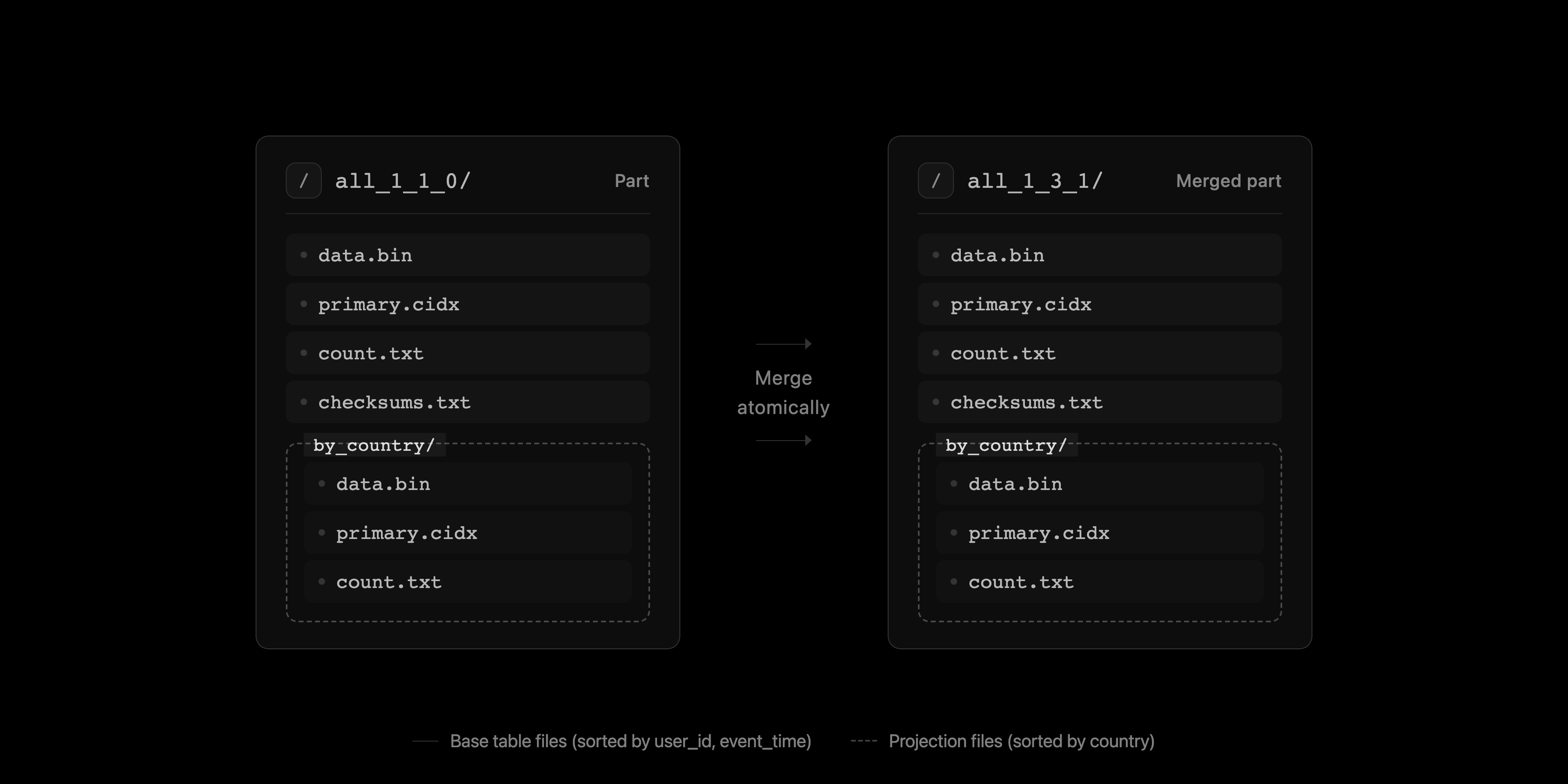
Base table files (sorted by user_id, event_time) and projection files (sorted by country) live side by side in the same part
The parent part's checksum includes the projection part's checksum, so integrity verification covers both.
Merges
This is the consistency guarantee that matters. Projection parts merge simultaneously with the main table parts, in the same merge operation.
There is no lag, the projection always has the same data as the source. This differs from materialized views, which fire on INSERT but can drift when you run mutations, lightweight deletes, or deduplication.
If you add a projection to an existing table, new parts get the projection automatically. Old parts don't. For old data, the optimizer always falls back to reading the base table, same as if the projection doesn't exist. You can materialize the projection for existing parts with:
ALTER TABLE web_analytics MATERIALIZE PROJECTION by_country;Until you run this, queries on old data won't benefit from the projection. This is the number one gotcha people hit: they add a projection, see no improvement, and assume projections are broken. Check system.projection_parts to see what's actually materialized.
Query routing
The optimizer evaluates projections per part at query time. For each part, it checks whether the projection has all the columns the query needs, estimates how many granules it would read from the base table vs the projection, and picks whichever option reads less data.
Multiple projections can cooperate on a single query for granule-level pruning. If you're running a previous version than v25.6, only one projection is evaluated per query.
You can verify which projection the optimizer picks:
EXPLAIN indexes = 1, projections = 1SELECT count()FROM web_analyticsWHERE country = 'DE';Two query settings let you override the optimizer when needed:
preferred_optimize_projection_namehints at a specific projectionforce_optimize_projection_nameforces it
Three types of projections
Not all projections store data the same way. A normal projection copies the full rows, an aggregate projection pre-computes GROUP BY results, and the most recent addition, index-only projections, stores almost nothing at all.
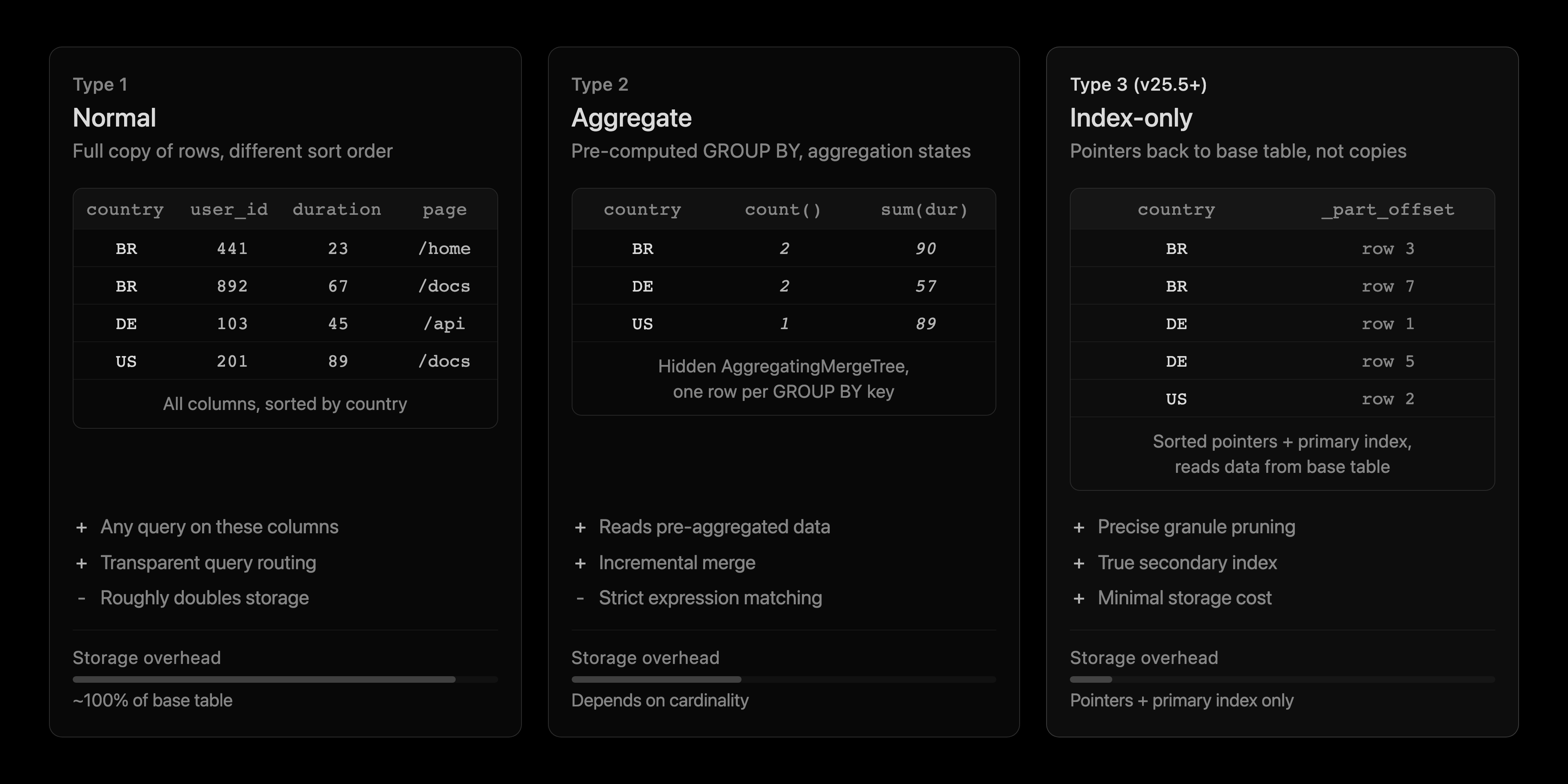
Three projection types with different storage and performance characteristics
Normal projections
The simplest type. Full copy of selected columns in a different sort order. The by_country example above is a normal projection.
Use case: your table is sorted by (user_id, event_time), but some queries filter by country. Instead of creating a materialized view that copies data to a separate table sorted by country, you add a projection. Same data, different order, automatic routing.
The cost is storage. A SELECT * projection roughly doubles the table size. You can reduce this by selecting only the columns you need:
PROJECTION country_duration ( SELECT country, duration ORDER BY country)This stores only country and duration in the projection, not the full row. Smaller, but queries that need other columns can't use it.
Aggregate projections
When you add a GROUP BY to a projection definition, ClickHouse creates a hidden AggregatingMergeTree under the hood. The projection stores intermediate aggregation states that get merged incrementally during background merges.
PROJECTION country_stats ( SELECT country, count(), sum(duration) GROUP BY country)A query like SELECT country, count(), sum(duration) FROM web_analytics GROUP BY country can be served entirely from this projection, reading pre-aggregated data instead of scanning all rows.
The internal mechanics are the same -State/-Merge pattern covered in the AggregatingMergeTree post and the materialized views deep dive. The difference is that ClickHouse manages everything: the state conversion, the incremental merges, and the query rewriting. You just define the GROUP BY.
There are limits. The query must match the projection's aggregate functions and GROUP BY columns. SELECT country, avg(duration) won't use a projection that only has count() and sum(duration), even though you could compute the average from those two. Expression matching is strict.
Index-only projections (v25.5+)
This is the last addition to the team. Index-only projections store almost nothing. Instead of copying data, an index-only projection stores just the sorting key and a _part_offset, a pointer back to the row's position in the base table part. ClickHouse uses the projection's primary index to find which granules contain matching rows, then reads the actual data from the base table.
PROJECTION by_country_idx ( SELECT _part_offset ORDER BY country)The storage overhead is minimal: just the country column values and the offsets, organized with their own primary index. Compare that to a normal projection that copies every column.
That is granule-level pruning. Instead of scanning the entire table, ClickHouse reads the projection's primary index to identify which 8,192-row granules contain matching rows, then reads only those granules from the base table.
v26.1 introduced a simplified syntax, the same behavior with less noise.
PROJECTION by_country INDEX country TYPE basicClickHouse already has skip indexes (bloom_filter, minmax, set, ngrambf_v1). How are index-only projections different?
Skip indexes attach statistical summaries to each granule. A minmax index stores the minimum and maximum value per granule. A bloom filter stores a probabilistic set membership structure. During query execution, ClickHouse checks the summary and skips granules that definitely don't match.
The word "definitely" is the key. Skip indexes have false positives. A minmax index on country knows the granule contains values between 'AT' and 'US', but if you're looking for 'DE', it can't skip that granule because 'DE' falls in range. A bloom filter might have a 1% false positive rate. These are fast and cheap, but approximate.
Index-only projections work differently. They re-sort the pointers by the projection's ORDER BY key and build a primary index over that sort order. The lookup is precise: ClickHouse navigates the primary index to find exactly which granules contain 'DE', with zero false positives.
| Skip indexes | Index-only projections | |
|---|---|---|
| Storage cost | Almost free (per-granule metadata) | Small (re-sorted pointers + primary index) |
| Pruning precision | Approximate (statistical summaries) | Precise (primary index lookup) |
| False positives | Yes | No |
| Write overhead | Minimal | Some (pointer materialization on INSERT) |
| Best for | Range filters, high-cardinality exclusion | Exact lookups, alternative sort orders |
When a skip index gives you 10x reduction but you need 1000x, an index-only projection is the next step up. When a bloom filter on a low-cardinality column skips 80% of granules but you need to skip 99.9%, the precise pruning of an index-only projection closes the gap.
The tradeoff is cost, since skip indexes are practically free. Index-only projections require storing and maintaining the re-sorted pointers. For most tables, start with skip indexes. If the pruning isn't selective enough, add an index-only projection.
Limitations and gotchas
Projections have hard boundaries.
The functional constraints are straightforward: no JOINs in projection definitions, no WHERE clauses (every row gets materialized), no chaining equivalent to cascading MVs, and no FINAL compatibility. Queries using FINAL bypass projections entirely, so if you're running ReplacingMergeTree or CollapsingMergeTree with FINAL, projections won't help.
Expression matching is strict. The query must use the same expressions as the projection definition. A projection with count() and sum(duration) won't be used by a query asking for avg(duration), even though the math is trivial.
Mutations are a separate concern. By default, lightweight deletes on tables with projections throw an error. Since v24.7, you can configure this with lightweight_mutation_projection_mode: throw (default), drop (drops projection parts, they rebuild on next merge), or rebuild (rebuilds immediately, slower).
The gotcha that catches most people: materialization is not automatic for existing data. Adding a projection only affects new inserts. Old data needs ALTER TABLE ... MATERIALIZE PROJECTION. On large tables, this is a heavy operation. Check progress in system.mutations.
Storage overhead depends on the type. Normal projections can double your table size. Aggregate projections are typically much smaller (one row per GROUP BY key combination). Index-only projections are the lightest. And projections share the parent table's TTL, so you can't expire projection data on a different schedule.
Projections vs materialized views: when to use which
The materialized views post had an 8-row comparison table. Here's the expanded version with the nuances that matter in practice.
| Projections | Materialized views | |
|---|---|---|
| What it does | Re-sorts or pre-aggregates existing data | Transforms, filters, joins, routes data |
| Table management | None (part of the source table) | Separate target table(s) to manage |
| Query changes | None (optimizer routes transparently) | Must query the target table directly |
| Filtering | No WHERE in definition | WHERE supported |
| JOINs | Not supported | Fully supported |
| Multi-stage pipelines | Not possible | Chain MVs freely |
| Consistency | Atomic (merge-level, never drifts) | INSERT-trigger only, can drift on mutations |
| Storage control | Shared with parent table | Independent engine, TTL, partitioning |
| Mutations | Problematic (needs special config) | Unaffected by source mutations |
| Backfill | MATERIALIZE PROJECTION | Manual INSERT INTO ... SELECT |
| Monitoring | Hard (hidden, requires EXPLAIN) | Easy (separate table, direct queries) |
| Write overhead | Part of the same write operation | Separate INSERT into target table |
The decision comes down to one question: does the data need to change shape?
If not, a projection handles it. Same data, different access path. If yes, that's a materialized view: JOINs, filtering, routing to a different engine, independent TTL.
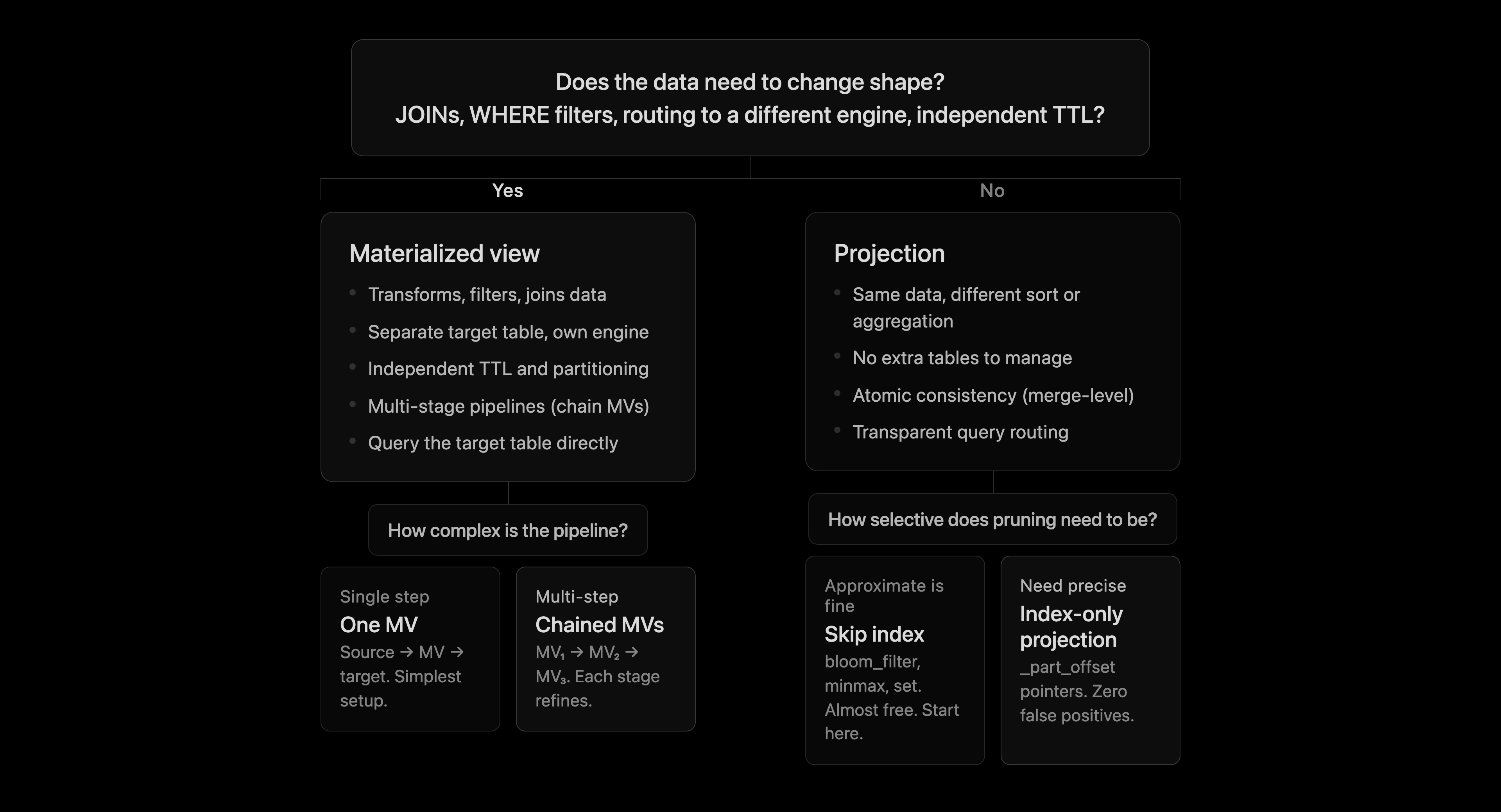
Decision framework for choosing between projections, skip indexes, and materialized views
Wrapping up
Projections are the quiet optimization tool without new tables to manage, and no query changes required. They handle the cases where your data is fine but your access pattern doesn't match the primary key. Index-only projections in v25.5+ make the storage argument weaker than it used to be.
Materialized views remain the right tool when data needs to change shape: JOINs, filtering, routing, independent lifecycles. The MV deep dive covers those patterns in depth.
Next in the series, we'll cover query optimization: what makes ClickHouse fast at the query level, and what kills it.